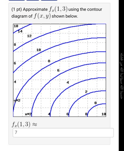
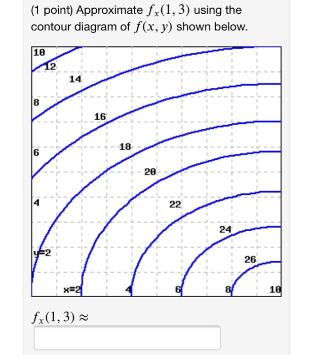
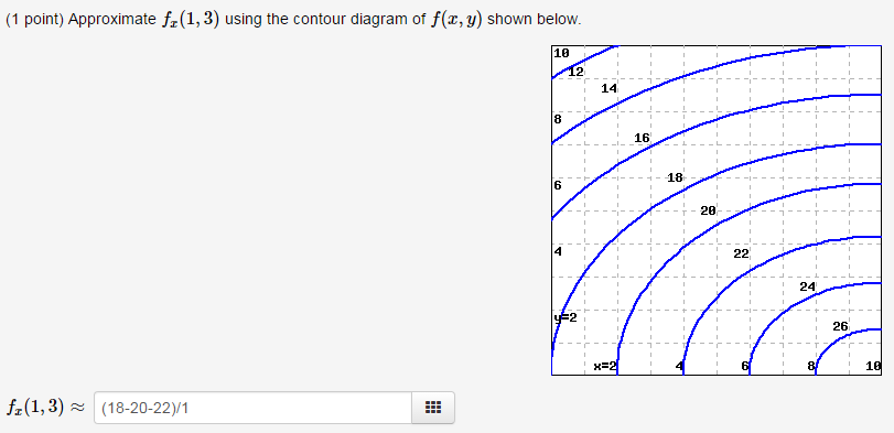
39 approximate fx(1,3) using the contour diagram of f(x,y) shown below.
It approximates a contour shape to another shape with less number of vertices depending upon the precision we specify. Now you can use this function to approximate the shape. Third image shows the same for epsilon = 1% of the arc length. Third argument specifies whether curve is closed... This article explains how backpropagation works in a CNN, convolutional neural network using the chain rule, which is different how it works in a perceptron. When we solve for the equations, as we move from left to right, ('the forward pass'), we get an output of f = -12.
It is shown that the known task of single-electron atom can be established with its own solution of fine-structure constant. Moreover, this approach may relate to electron transition directly to the proton structure, that with a hyper-fine structure like the Lamb shift of hydrogen atom is specifically associated.
Approximate fx(1,3) using the contour diagram of f(x,y) shown below.
You are using an out of date browser. It may not display this or other websites correctly. You should upgrade or use an alternative browser. Let ##X## be a topological space so that, for any topological space ##Y##, any map ##f:X\longrightarrow Y## is continuous. The following technique for approximating the characteristic function of intervals in $[0,1]$ using Fourier series with coefficients having inverse quadratic decay is given in the book Diophantische Approximationen (Ergebnisse der Math., IV, 4; Berlin, 1936) by J.F.Koksma. The Fill method computes the bin number corresponding to the given x, y or z argument and increments this bin by the given weight. The Fill() method returns the bin number for 1-D histograms or global bin number for 2-D and 3-D histograms.
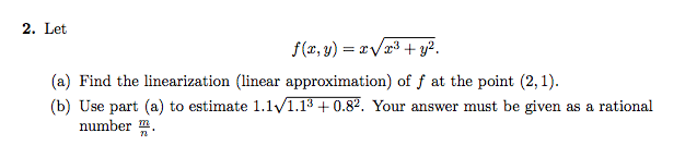
Approximate fx(1,3) using the contour diagram of f(x,y) shown below.. Using contour detection, we can detect the borders of objects, and localize them easily in an image. It is often the first step for many interesting applications, such as image-foreground extraction, simple-image segmentation, detection and recognition. So let's learn about contours and contour detection... The calculator will find the linear approximation to the explicit, polar, parametric, and implicit curve at the given point, with steps shown. If the calculator did not compute something or you have identified an error, or you have a suggestion/feedback, please write it in the comments below. The block diagram of the proposed approach is shown in Figure 1. The first step is preprocessing by 2.3.1. Initial curve The active contour method starts with an initial curve. The shape of the initial curve is The proposed algorithm develops an equation below for modification of evolution function We use three different estimators to fit the function: linear regression with polynomial features of degree 1, 4 and 15. However, you should only collect more training data if the true function is too complex to be approximated by an estimator with a lower variance.
The left hand side is a double integral. In particular, it is the integral of $f_X(t)$ over the shaded region in Figure 4.4. Although $g$ is not monotone, it can be divided to a finite number of regions in which it is monotone. Thus, we can use Equation 4.6. In approximating contours, a contour shape is approximated over another contour shape, which may be not that much similar to the first contour shape. For approximation we use approxPolyDP function of openCV which is explained below. Given the residuals f(x) (an m-D real function of n real variables) and the loss function rho(s) (a scalar function), least_squares If the argument x is complex or the function fun returns complex residuals, it must be wrapped in a real function of real arguments, as shown at the end of the Examples section. A. –1.26 B. –2.52 C. –9.64 D. –12.00 The answer to this practice diploma question is -1.26 but I'm not sure as to why that is. Thank you for any clarification.
Page: 5. The state diagram has two states State 0 : Output = Input State1 : Output = Complement of input PS Inp. NS Out A xAy 0 000 0 111 1 011 1 110 DA= A + x y=A⊕x. 5-19) A sequential circuit has three flip-flops A, B, C; one input x; and one output, y. The state diagram is shown in Fig.P5-19. It would be absolutely amazing if the chart could dynamically update the spacing according to the two middle (X, Y) values. ​ For reference: [https://imgur.com/a/yKJ0FRA](https://imgur.com/a/yKJ0FRA) ANSWER System.out.print(a); System.out.print(b); System.out.print(c + " "); System.out.print(a); System.out.print(c); System.out.print(b + " "); System.out.print(b); System.out.print(a); System.out.print(c + " "); System.out.print(b); System.out.print(c); System.out.print(a + " "); System.out.print(c); System.out.print(a); System.out.print(b + " "); System.out.print(c); System.out.print(b); System.out.print(a); As the title says i'm trying to make a diagram. Excel is not recognizing my data. I have tried opening and closing the select data menu many times, reselecting it, deleting it all and adding it back and it has not helped so far. The data is imported from a CSV dump from a database.\[Image for clarity\]([https://imgur.com/NhYLx2Z](https://imgur.com/NhYLx2Z)) Extra info: Windows 10 desktop Excel 365 in Dutch
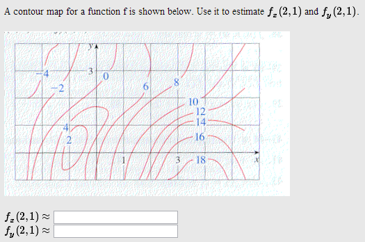
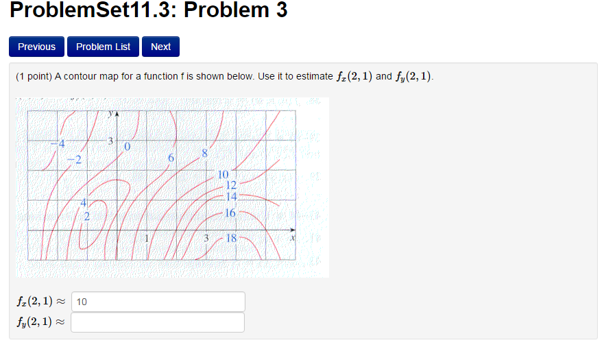
Solved: A Contour Map For A Function F Is Shown Below. Use ...
SkewT-logP diagram: using transforms and custom projections. You can use tuple-unpacking also in 2D to assign all subplots to dedicated variables fig, (ax1, ax2) = plt.subplots(2, sharex=True) fig.suptitle('Aligning x-axis using sharex') ax1.plot(x, y) ax2.plot(x + 1, -y).
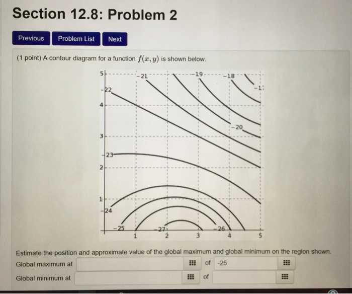
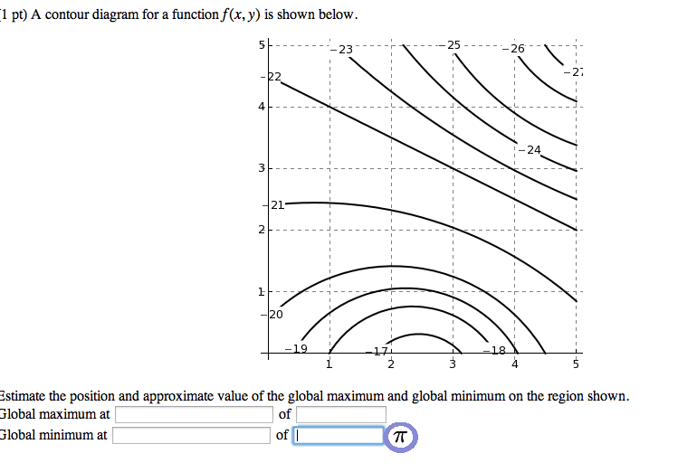
Solved: A Contour Diagram For A Function F(x, Y) Is Shown ...
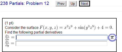
-2 Figure P3.3-1 (b) Express the following sequence as a sum of step functions, i.e., in the form. s[n] = ( aku[n - k]. P3.5 Consider the three systems H, G, and F defined in Figure P3.5-1.
Solved: (1 Pt) Approximate Fr (1,3) Using The Contour 1 Pt ...
I’m having difficulty working out how to start on this question, I don’t want an answer I just want to be pointed in the right direction
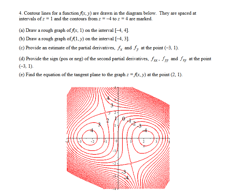
Solved: Contour Lines For A Function F(x, Y) Are Drawn In ...
Academia.edu is a platform for academics to share research papers.
Solved: I've Tried This Problem Several Times And Dont Rea ...
Free Linear Approximation calculator - lineary approximate functions at given points step-by-step. This website uses cookies to ensure you get the best experience. By using this website, you agree to our Cookie Policy.
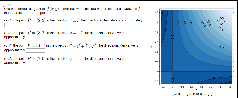
Solved: Use The Contour Diagram For F(x, Y) Shown Below To ...
Use differentials to approximate the maximum percentage error in the calculated area. Show transcribed image textSuppose that a function f(x, y, z) is differentiated the point (0, -1, -2) and L(x, y, z) = x + 2y is the local linear approximation to f Find f(0, -1, -2), fx(0, -1, -2) fy(0, -1, -2) fz(0, -1, -2). A...
Solved: A Contour Diagram For The Functions Z = F(x,y) Is ...
(A) shows the block diagram representation of a control system. When this system is excited with a unit step input, it responds as shown in the graph of Fig (B). Find, 1- The overall transfer function C(s)y/R(s). 2- The damping ratio g 3- The natural undamped frequency o 4- The damped natural...
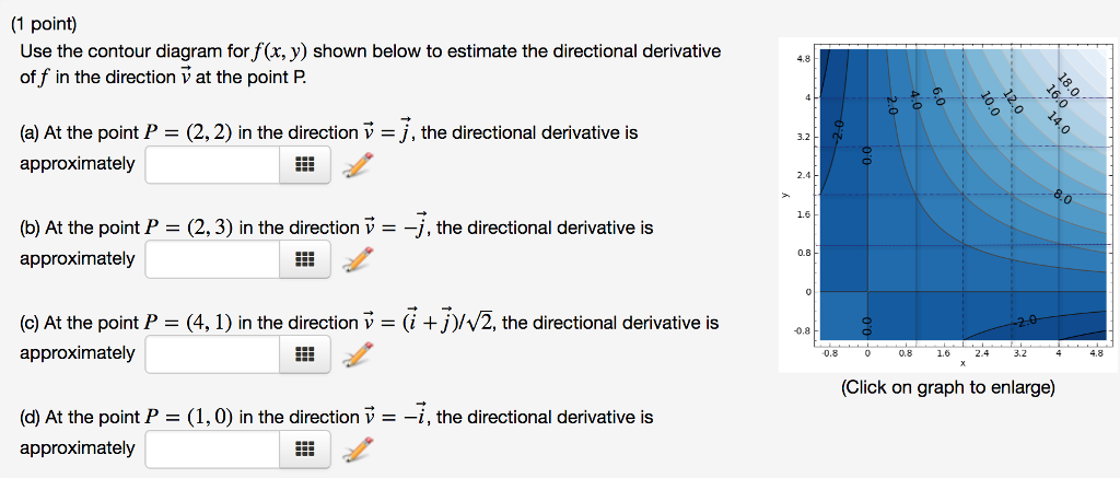
Solved: Use The Contour Diagram For F(x, Y) Shown Below To ...
​ https://preview.redd.it/yqvr84wwhdx61.png?width=532&format=png&auto=webp&s=dd58430a789ed81bdb80d32e1354ed619ec18a8e

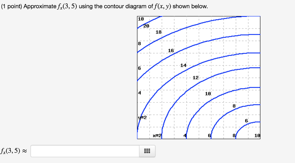
Solved: Approximate Fx(3,5) Using The Contour Diagram Of F ...
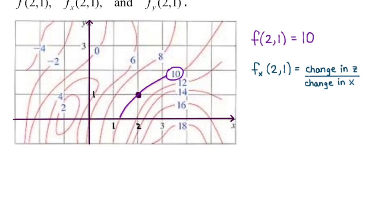
The following diagram illustrates these problems. There are certain things you must remember from College Algebra (or similar classes) when solving for the equation of a The equation for the slope of the tangent line to f(x) = x2 is f '(x), the derivative of f(x). Using the power rule yields the following
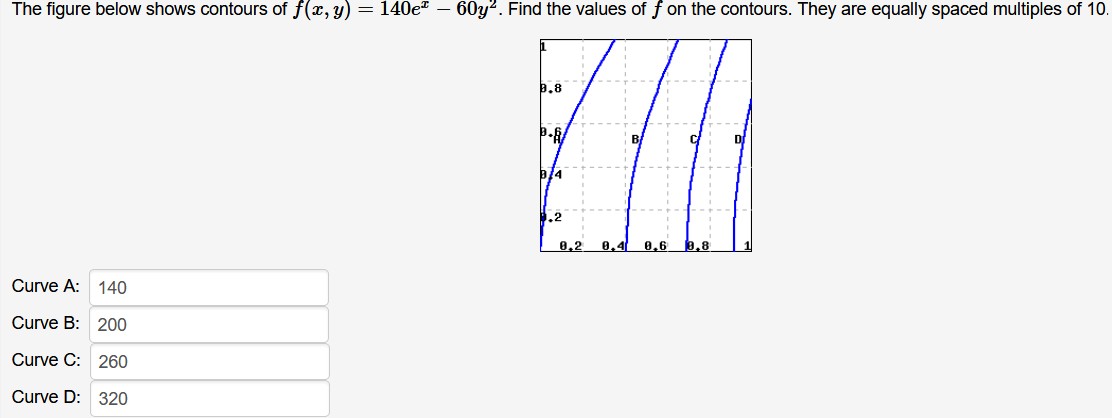
Answered: The figure below shows contours of f(x,… | bartleby
This MATLAB function creates a contour plot containing the isolines of matrix Z, where Z contains height values on the x-y plane. Define Z as a function of two variables, X and Y. Then create a contour plot of that function, and display the labels by setting the ShowText property to 'on'.

Eckhard Bick - PDF Free Download
where big-O notation is used, combining the equations above yields the approximation formula in its logarithmic form De Moivre gave an approximate rational-number expression for the natural logarithm of the constant. Stirling's contribution consisted of showing that the constant is precisely.

Solved: Approximate Fx(1,3)fx13 Using The Contour Diagram ...
1. Make predictions about your future. Use the future continuous, affirmative or negative form of the verbs in brackets. 2. Look at the timeline for a new medical school. Write sentences using the affirmative or negative form of the future perfect and the prompts below.

Solved: A Contour Diagram For A Function F(x,y) Is Shown B ...
This calculator solves Systems of Linear Equations using Gaussian Elimination Method, Inverse Matrix Method, or Cramer's rule. Leave cells empty for variables, which do not participate in your equations. To input fractions use /: 1/3.
A Contour Map Is Given For A Function F Use It To Estimate ...
From a hilltop, the horizon lies below the horizontal level at an angle called the "dip". Kepler was unable to construct an accurate model using polygons, but he noted that, if successive polygons with an increasing number of Schematic diagram of some key physical processes in the climate system.
Solved: (1 Point) Approximate Fx(1,3) Using The Contour Di ...
I have arrays x = \[ ...\], y = \[ ...\], and f = \[ ... \]. How can I make a contour plot (2D plot) for these? Thank you!

Users Guide 5 - PDF Free Download
We use the Newton's method. problem number 19 toe Approximate route are of the given function F and the initial approximation X note. The formula that we use for this is X and plus one is equal to x n minus. F of x n over f dash of its and now case off our backs equals sign.
A Contour Map Is Given For A Function F Use It To Estimate ...
Method 1 (Use recursion) A simple method that is a direct recursive implementation mathematical recurrence relation given above. Method 2 (Use Dynamic Programming) We can avoid the repeated work done in method 1 by storing the Fibonacci numbers calculated so far.
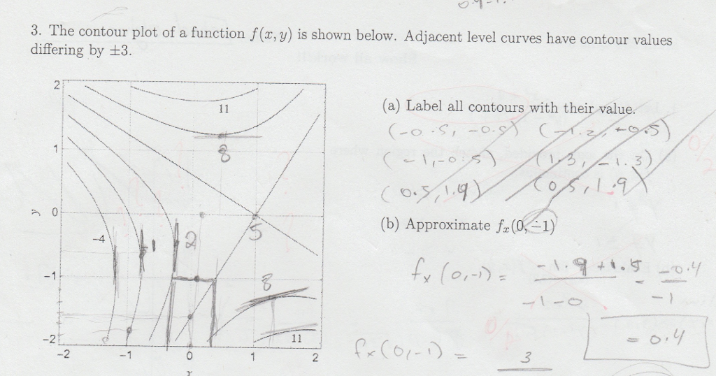
Solved: 3. The Contour Plot Of A Function F(x, Y) Is Shown ...
Below is a mathematical representation of a neuron. The different components of the neuron are Which of the following is true about model capacity (where model capacity means the ability of neural network to approximate complex functions) ? The below graph shows the accuracy of a trained...

A Contour Map Is Given For A Function F Use It To Estimate ...
I think that this is a straightforward question but how can we rewrite g(x)=f(x-4)+3 so that it is easier to solve the question? thank you
Solved: Approximate Fx(1,3) Using The Contour Diagram Of F ...
We use cookies to improve your experience on our site and to show you relevant advertising. By browsing this website, you agree to our use of cookies. root of an equation using Secant method. f(x) =. Find Any Root Root Between and.
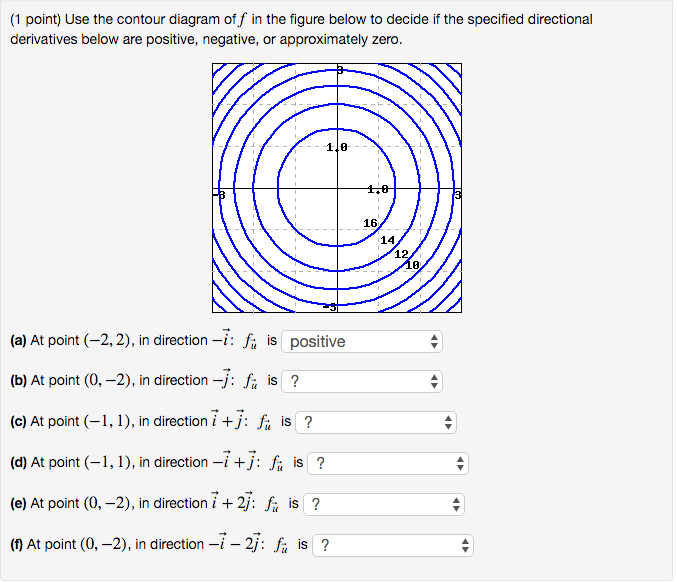
Solved: Use The Contour Diagram Of F In The Figure Below T ...
examples and problems in mechanics of materials stress-strain state at a point of elastic deformable solid editor-in-chief yakiv karpov
A Contour Map Is Given For A Function F Use It To Estimate ...
The Fill method computes the bin number corresponding to the given x, y or z argument and increments this bin by the given weight. The Fill() method returns the bin number for 1-D histograms or global bin number for 2-D and 3-D histograms.
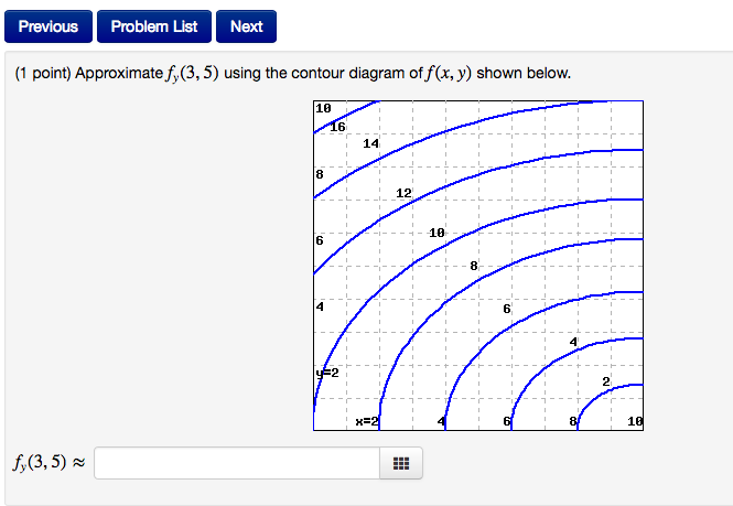
Solved: Approximate F_y(3, 5) Using The Contour Diagram Of ...
The following technique for approximating the characteristic function of intervals in $[0,1]$ using Fourier series with coefficients having inverse quadratic decay is given in the book Diophantische Approximationen (Ergebnisse der Math., IV, 4; Berlin, 1936) by J.F.Koksma.

Solved: Approximate Fx(1,3) Using The Contour Diagram Of F ...
You are using an out of date browser. It may not display this or other websites correctly. You should upgrade or use an alternative browser. Let ##X## be a topological space so that, for any topological space ##Y##, any map ##f:X\longrightarrow Y## is continuous.
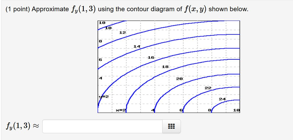
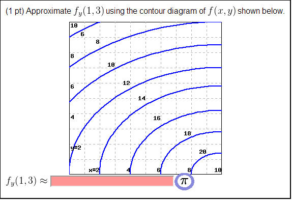
Solved: Approximate F_y (1, 3) Using The Contour Diagram O ...
Approximate Fy( 1,3) Using The Contour Diagram Of ...

(1 point) A contour diagram for a function f(x,y) is shown ...

複線ãƒã‚¤ãƒ³ãƒˆãƒ¬ãƒ¼ãƒ«â‘£: SketchUpã§ãƒ—ラレール

A Contour Map Is Given For A Function F Use It To Estimate ...

Eckhard Bick - PDF Free Download
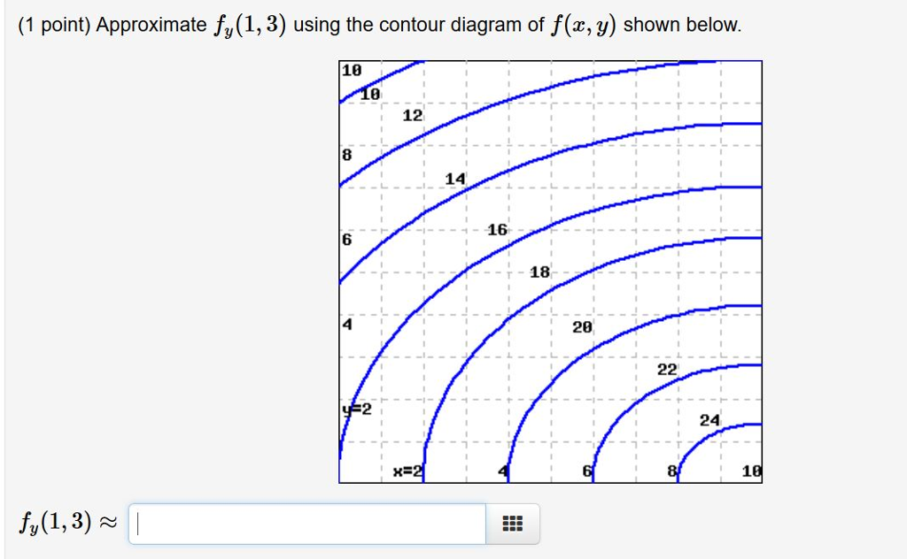
Solved: Approximate Fy(1,3) Using The Contour Diagram Of F ...
Solved: A Contour Diagram For A Function F(x,y) Is Shown B ...
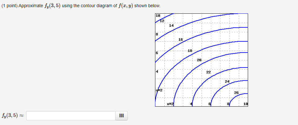
Solved: (1 Point) Approximate Fy (3,5) Using The Contour D ...
Solved: (1 Point) Approximate Fs(3,5) Using The Contour Di ...
Approximate Fy( 1,3) Using The Contour Diagram Of ...
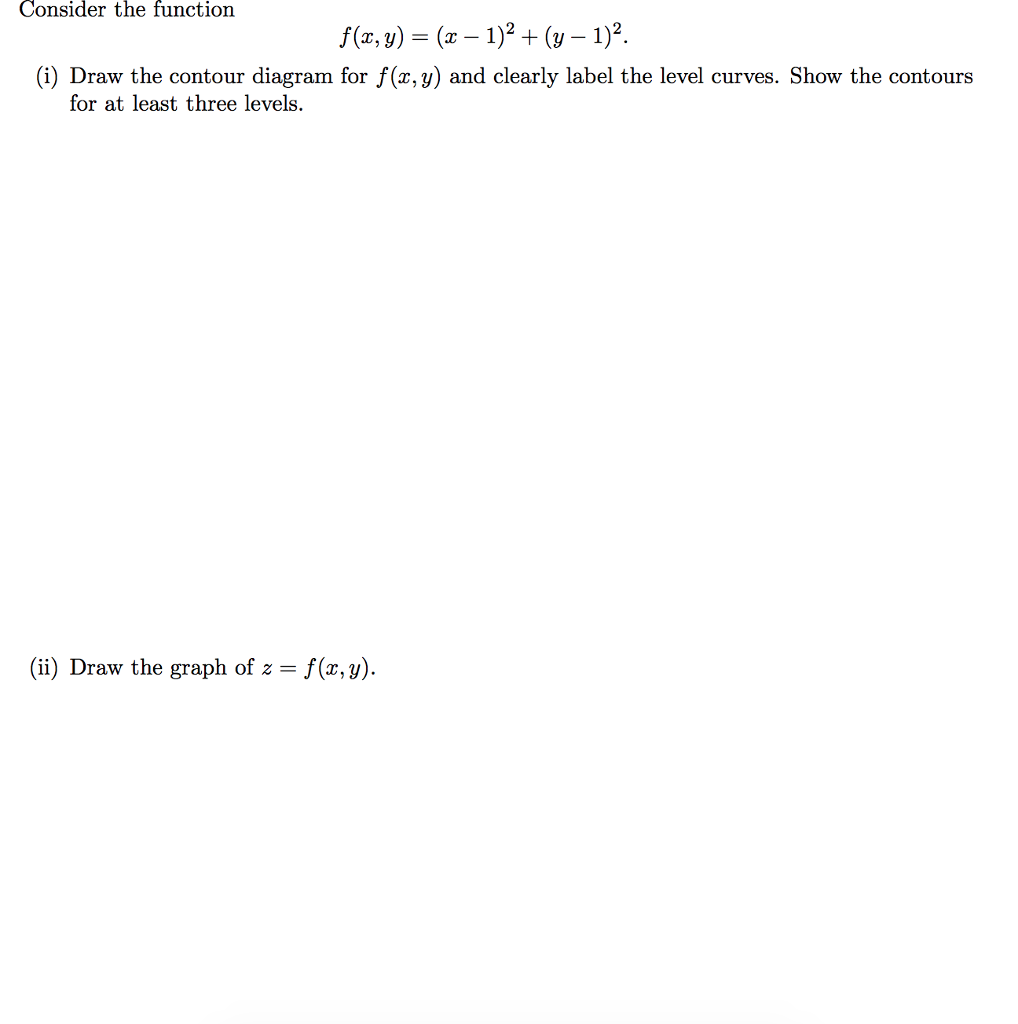
Consider the functio (i) Draw the contour diagram for ...
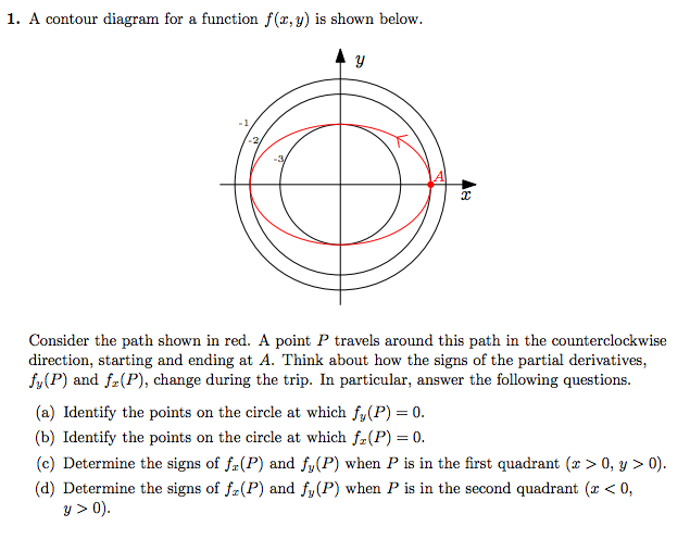
Solved: A Contour Diagram For A Function F(x,y) Is Shown B ...
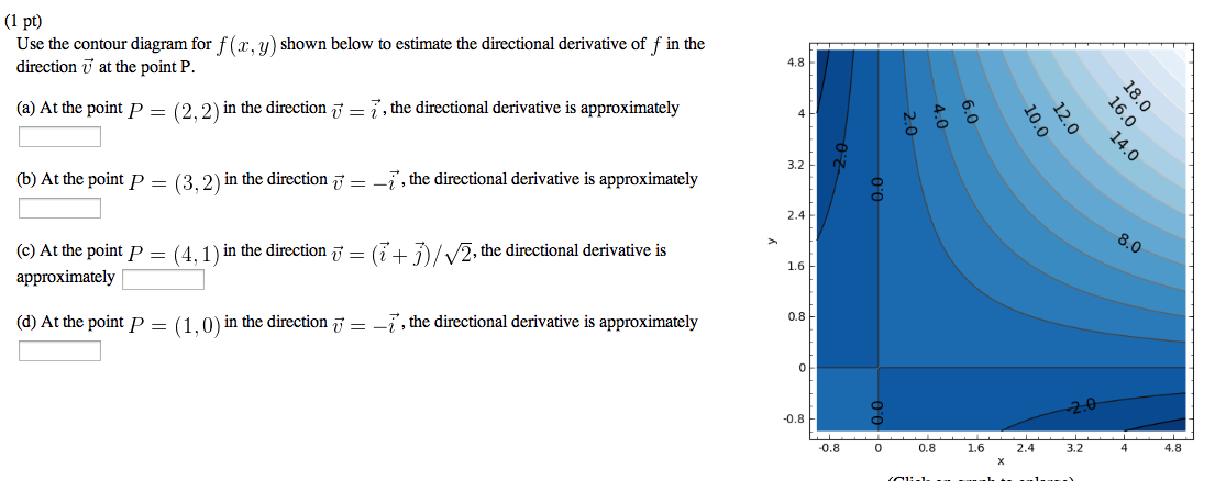
Solved: Use The Contour Diagram For F(x, Y) Shown Below To ...

Users Guide 5 - PDF Free Download
0 Response to "39 approximate fx(1,3) using the contour diagram of f(x,y) shown below."
Post a Comment